Reading and using the SLSTR MDB files¶

By design, the content of SLSTR matchups is very rich and it can be overwhelming. This primer is intended for support you in this (relatively) steep initial learning curve.

We will start exploring and understand the content of MDB files with simple netCDF4 and numpy functions which have to be installed in your environment.

basics¶

Let’s first open a sample file, containing match-ups with CMEMS drifters:

import netCDF4 as netcdf

# open file
mdbfile = netcdf.Dataset('/home/cercache/project/s3vt/2016/287/S3A_SL_2_WCT_cmems_drifter_20161013000000_20161013060000.nc')

The file contains a lot of variables! The following examples will help you to understand and analyse the content of the match-up files. Further in this tutorial, more advanced function usage from s3mdbpackage are provided.

The main file dimension is time : it gives the number of match-ups. Let’s get the number of match-ups from our example file

print len(mdbfile.dimensions['time'])

The time, lat and lon variables gives the locations and times of all our match-ups. They correspond to the locations and times of the closest in situ measurement to satellite pixels. These arrays have as many values as the number of match-ups:

# get latitudes of match-ups
lat = mdbfile.variables['lat'][:]

# print number of lat values
print len(lat)

# this is the latitude of matchup #3 in the file:
print lat[3]

32.207

understanding the in situ section of the matchups¶

The variables with in situ measurements will be prefixed with cmems_drifter__

for var in mdbfile.variables:
    if 'cmems_drifter__' in var:
        print var

cmems_drifter__origin
cmems_drifter__dynamic_target_center_index
cmems_drifter__lon
cmems_drifter__quality_level_4
cmems_drifter__rejection_flag_4
cmems_drifter__quality_level_1
cmems_drifter__rejection_flag_3
cmems_drifter__quality_level_3
cmems_drifter__quality_level_2
cmems_drifter__meas_depth_4
cmems_drifter__rejection_flag_2
cmems_drifter__time
cmems_drifter__meas_depth_0
cmems_drifter__meas_depth_1
cmems_drifter__meas_depth_2
cmems_drifter__meas_depth_3
cmems_drifter__rejection_flag_0
cmems_drifter__rejection_flag_1
cmems_drifter__lat
cmems_drifter__water_temperature_3
cmems_drifter__water_temperature_2
cmems_drifter__water_temperature_1
cmems_drifter__water_temperature_0
cmems_drifter__water_temperature_4
cmems_drifter__quality_level_0
cmems_drifter__climatology_water_temperature
cmems_drifter__solar_zenith_angle

Most in situ variables have two dimensions: time and cmems_drifter___time

print mdbfile['cmems_drifter__water_temperature_0'].dimensions

(u'time', u'cmems_drifter___time')

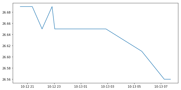
the reason for the the extra dimension cmems_drifter___time is that we provide the history of the buoy for each match-up in a time window of +/- 6 hours around the match-up time:

# get the buoy temperature history of our match-up #3
temp = mdbfile['cmems_drifter__water_temperature_0'][3, :]

# get the corresponding time of each temperature measurement
times = mdbfile['cmems_drifter__time'][3, :]


# because all buoys don't have the same sampling rate, the number of measurements in the buoy history
# vary from one match-up to another. Therefore, the end of the history array is often trailed with
# fill values.
print times

[1129148880 1129151580 1129151940 1129152120 1129154760 1129157460
 1129158180 1129160280 1129160580 1129162680 1129163160 1129165920
 1129166220 1129168560 1129171980 1129181640 1129187700 1129189380 -- -- --
 -- -- -- -- -- -- -- -- -- -- -- -- -- -- -- -- -- -- -- -- -- -- -- -- --
 -- -- -- -- -- -- -- -- -- -- -- -- -- -- -- -- -- -- -- -- -- -- -- -- --
 -- -- -- -- -- -- -- -- -- -- -- -- -- -- -- -- -- -- -- -- -- -- -- -- --
 -- -- -- -- -- -- -- -- -- -- -- -- -- -- -- -- -- -- -- -- -- -- -- -- --
 -- -- -- -- -- -- -- -- -- -- -- -- -- -- -- -- -- -- -- -- --]

%matplotlib inline
import numpy

# Let's get rid of these trailing file values
times = numpy.ma.fix_invalid(times).compressed()
temp = numpy.ma.fix_invalid(temp).compressed()

# transform these time values in datetime objects
times = netcdf.num2date(times, mdbfile['cmems_drifter__time'].units)

# display this temperature time series
from matplotlib import pyplot

fig = pyplot.figure(figsize=(10,5))
pyplot.plot(times, temp)
pyplot.show()

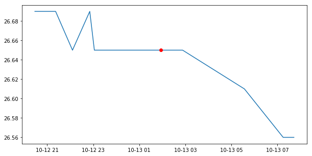
The closest measurement in time to satellite pixels in this time series, is given by the variable cmems_drifter__dynamic_target_center_index. Here for our match-up #3:

indice = mdbfile['cmems_drifter__dynamic_target_center_index'][3]
print indice

# the closest temperature value is then:
print mdbfile['cmems_drifter__water_temperature_0'][3, indice]

26.6499996185

# verify on above plot that is at the center of the history
fig = pyplot.figure(figsize=(10,5))
pyplot.plot(times, temp)
pyplot.plot(times[indice], temp[indice], color='r', marker="o")
pyplot.show()

Some variables have a _0, _1, _2, _3, _4 suffix. They correspond to different depth levels, as the first 5 depth level measurement were retained for any in situ source : this is not the actual depth value, just the rank, 0 being the closest to surface and 4 the deepest.

For drifters, there will be most likely only a single value in <field>_0 and fill values in other levels, except for the few who may measure the water temperature at different levels.

# print closest temperature value to surface for match-up #3
print mdbfile.variables['cmems_drifter__water_temperature_0'][3, indice]

26.6499996185

# this drifter provides only a single depth measurement
print mdbfile.variables['cmems_drifter__water_temperature_1'][3, indice]

--

# note that the actual depth (when available at in situ provider) is provided in the corresponding depth field
print mdbfile.variables['cmems_drifter__meas_depth_0'][3, indice]

0.0

The handy read_insitu_field function from s3analysis package allow to retrieve a multi-dimensional array instead of reading separately each level field. Just query the name of the field with the _<x> suffix and set the closest_to_surface argument to False. See some examples further.

# get full profiles in one single array
closest_value = read_insitu_field(mdbfile, 'cmems_drifter__water_temperature', closest_to_surface=False)
print closest_value.shape

(488, 5)

understanding the satellite part of the matchups¶

The MDB is a multi-dataset match-up database: for each match-up, a full stack of fields from each of these datasets is provided (filled with fill values when they were not available or not in the match-up window).

The fields from each dataset is prefixed with <dataset id>__.

For instance, to get the fields from S3A_SL_2_WST product only:

for var in mdbfile.variables:
    if 'S3A_SL_2_WST__' in var:
        print var

S3A_SL_2_WST__dynamic_target_distance
S3A_SL_2_WST__dynamic_target_center_index
S3A_SL_2_WST__origin
S3A_SL_2_WST__dynamic_target_time_difference
S3A_SL_2_WST__time
S3A_SL_2_WST__nadir_sst_theoretical_uncertainty
S3A_SL_2_WST__sses_standard_deviation
S3A_SL_2_WST__wind_speed_dtime_from_sst
S3A_SL_2_WST__l2p_flags
S3A_SL_2_WST__dt_analysis
S3A_SL_2_WST__aerosol_dynamic_indicator
S3A_SL_2_WST__dual_nadir_sst_difference
S3A_SL_2_WST__lon
S3A_SL_2_WST__sst_theoretical_uncertainty
S3A_SL_2_WST__miniprod_content_mask
S3A_SL_2_WST__lat
S3A_SL_2_WST__wind_speed
S3A_SL_2_WST__sea_ice_fraction_dtime_from_sst
S3A_SL_2_WST__adi_dtime_from_sst
S3A_SL_2_WST__brightness_temperature
S3A_SL_2_WST__sea_ice_fraction
S3A_SL_2_WST__nedt
S3A_SL_2_WST__sses_bias
S3A_SL_2_WST__quality_level
S3A_SL_2_WST__sst_algorithm_type
S3A_SL_2_WST__sea_surface_temperature
S3A_SL_2_WST__satellite_zenith_angle

Each satellite match-up is provided as box : the match-up pixel and its neighbours within a 21x21 pixel box).

# display the content of S3A_SL_2_WST__wind_speed for matchup #3
sst = mdbfile.variables['S3A_SL_2_WST__wind_speed'][3, :, :]
pyplot.imshow(sst, interpolation='nearest')
pyplot.show()

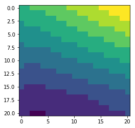
The central pixel of the box is the closest to the in situ measurement.

# get the lat/lon of the box for S3A_SL_2_WST dataset, for our match-up #3
lat = mdbfile.variables['S3A_SL_2_WST__lat'][3, :, :]
lon = mdbfile.variables['S3A_SL_2_WST__lon'][3, :, :]

# display the location of all pixels from the box
fig = pyplot.figure(figsize=(8,8))
pyplot.scatter(lat, lon, marker='+', color='b')

# highlight the center pixel
pyplot.plot(lat[10, 10], lon[10, 10], marker='o', color='r')

# overlay the in situ centre pixel and verify it is the closest to the pixel center
pyplot.plot(mdbfile.variables['lat'][3], mdbfile.variables['lon'][3], color='g', marker='o')

# display
pyplot.show()

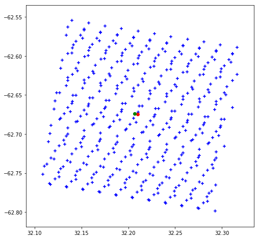
In some cases, the in situ measuement is not centred on the central pixel, this is because the in situ measurement is out of the footprint of input satellite file (granule). These shifted boxes can be easily spotted by using the distance between the central pixel and the in situ measurement, S3A_SL_2_WST__dynamic_target_distance : they will have a value greater than 1000m.

# number of match-ups
print len(mdbfile.variables['time'])

# print maximum match-up distance, in meters, found for these match-ups
print mdbfile.variables['S3A_SL_2_WST__dynamic_target_distance'][:].max()

import numpy

# mask match-ups where the distance to satellite pixel  is greater than 1km
pixel_distance = mdbfile.variables['S3A_SL_2_WST__dynamic_target_distance'][:]

times = mdbfile.variables['time'][:]
times = numpy.ma.masked_where(pixel_distance > 1000., times)

# number of remaining match-ups
print times.count()

Similarly, the time difference between the satellite pixels and the closest in situ measurement in time, provided by S3A_SL_2_WST__dynamic_target_time_difference can be used as a filtering criteria (the colocation window is 2h for drifters and moored buoys, 12h for argo floats):

time_difference = mdbfile.variables['S3A_SL_2_WST__dynamic_target_time_difference'][:]

# select match-ups which time difference is lower than 1h
times = mdbfile.variables['time'][:]
times = numpy.ma.masked_where(time_difference > 3600, times)

# number of remaining match-ups
print times.count()

Many satellite match-ups are also actually cloudy and don’t have a valid SST value. However there may be some neighbouring pixel in the box with a valid SST value. If it is close enough, you may want to keep it in your analysis. For instance, let’s take this cloudy match-up:

# Here is an example of cloudy match-up
sst = mdbfile.variables['S3A_SL_2_WST__sea_surface_temperature'][15, :, :]

#quality = mdbfile.variables['S3A_SL_2_WST__quality_level'][15, :, :]
pyplot.imshow(sst, interpolation='nearest')
pyplot.show()

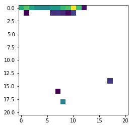
# print the central value => it is masked (invalid)
print sst[10, 10]

--

Note that for all other than SLSTR datasets in the match-ups, resampling on the SLSTR product grid was performed using closest neighbour regridding.

traceability¶

All match-ups can be traced back to their original file, using the <dataset>__origin and <dataset>__dynamic_target_center_index fields

# get the source granule file for our match-up #3
print mdbfile.variables['S3A_SL_2_WST__origin'][3]

S3A_SL_2_WST____20161013T021744_20161013T022044_20161013T043834_0179_009_360______MAR_O_NR_002.SEN3

# get the row and column indices of the match-up pixel in this file
print mdbfile.variables['S3A_SL_2_WST__dynamic_target_center_index'][3]

[1151  257]

some advanced functions with `s3analysis`¶

the s3analysis packages provides an abstraction layer of the individual MDB files and some more advanced function to ease the extraction and analysis of information.

In additional to helper functions described above, two more functions are provided: * read_satellite_data * read_insitu_data

The main usage of these function is to loop over the match-up files of time range and return a concatenated result. So you don’t have to bother with iterating over files and messing with arrays, these function do that for you!

note: these functions assume you stored the MDB files as they are on Ifremer repository, stored by ``year`` and ``day in year`` folders!

Let’s start with read_satellite_data helper function:

from s3analysis.slstr.mdb.slstrmdb import SLSTRMDB
import datetime

# instantiate the class to read MDB data
mdb = SLSTRMDB(config={
    'mdb_output_root': "/home/cercache/project/s3vt/",
    'reference': 'S3A_SL_2_WST'
})

# extraction criteria
start = datetime.datetime(2016, 10, 13)
source = 'cmems_drifter'

# fields to read (use the original field names from the source SLSTR products)
fields = {
    'S3A_SL_2_WST': ['sea_surface_temperature', 'quality_level']
}

# perform the data selection for day 13 Oct 2016. By default it returns the closest pixel only.
res = mdb.read_satellite_data(source, start, dataset_fields=fields, reference='S3A_SL_2_WST')

# number or match-ups
print res['S3A_SL_2_WST']['sea_surface_temperature'].size

# number of valid (unmasked) match-ups
print res['S3A_SL_2_WST']['sea_surface_temperature'].count()

Reading file 4 over 4
2113
910

# Among the returned values, we can also filter out those who are two far from the in situ measurement,
# using the ``max_distance`` threshold, in meter
res = mdb.read_satellite_data(source, start, dataset_fields=fields, max_distance=3000)
print res['S3A_SL_2_WST']['sea_surface_temperature'].count()

Reading file 4 over 4
913

# you can also provide a time range instead of a single day, by specifying the end date
# in ``end`` argument
end = datetime.datetime(2016, 10, 14)
res = mdb.read_satellite_data(source, start,  dataset_fields=fields, end=end)

# number or match-ups
print res['S3A_SL_2_WST']['sea_surface_temperature'].count()

Reading file 8 over 8
1827

You can also get instead request the closest valid measurement, where the validity is defined by some selection filter

res = mdb.read_satellite_data(source, start,  dataset_fields=fields, filters={'S3A_SL_2_WST': {'quality_level': [3, 5]}})

# number or match-ups
print res['S3A_SL_2_WST']['sea_surface_temperature'].count()

Reading file 4 over 4
1

The s3analysis package provides a handy function to only retrieve the closest in situ value (in time) from each match-up at once : read_insitu_data

# extraction criteria
insitu_fields = ['water_temperature']

# perform the data selection for day 13 Oct 2016
res = mdb.read_insitu_data(source, start, insitu_fields)

# this returns by default the closest valid measurement to surface for each match-up
# in each profile as seen in the dimensions of the returned result
print res['water_temperature'].shape

# number or match-ups
print res['water_temperature'].count()

# alternatively, you can also select the whole profile by deactivating the surface selection
res = mdb.read_insitu_data(source, start, insitu_fields, closest_to_surface=False)

print res['water_temperature'].shape

File: /home/cercache/project/s3vt/2016/287/S3A_SL_2_WCT_cmems_drifter_20161013180000_20161014000000.nc
File: /home/cercache/project/s3vt/2016/287/S3A_SL_2_WCT_cmems_drifter_20161013120000_20161013180000.nc
File: /home/cercache/project/s3vt/2016/287/S3A_SL_2_WCT_cmems_drifter_20161013060000_20161013120000.nc
File: /home/cercache/project/s3vt/2016/287/S3A_SL_2_WCT_cmems_drifter_20161013000000_20161013060000.nc
(2113,)
2113
File: /home/cercache/project/s3vt/2016/287/S3A_SL_2_WCT_cmems_drifter_20161013180000_20161014000000.nc
File: /home/cercache/project/s3vt/2016/287/S3A_SL_2_WCT_cmems_drifter_20161013120000_20161013180000.nc
File: /home/cercache/project/s3vt/2016/287/S3A_SL_2_WCT_cmems_drifter_20161013060000_20161013120000.nc
File: /home/cercache/project/s3vt/2016/287/S3A_SL_2_WCT_cmems_drifter_20161013000000_20161013060000.nc
(2113, 5)

# Similarly you can also provide a time range instead of a single day, by specifying the end date
# in ``end`` argument
end = datetime.datetime(2016, 10, 14)
res = mdb.read_insitu_data(source, start, insitu_fields, end=end)

# number or match-ups
print res['water_temperature'].count()

File: /home/cercache/project/s3vt/2016/287/S3A_SL_2_WCT_cmems_drifter_20161013180000_20161014000000.nc
File: /home/cercache/project/s3vt/2016/287/S3A_SL_2_WCT_cmems_drifter_20161013120000_20161013180000.nc
File: /home/cercache/project/s3vt/2016/287/S3A_SL_2_WCT_cmems_drifter_20161013060000_20161013120000.nc
File: /home/cercache/project/s3vt/2016/287/S3A_SL_2_WCT_cmems_drifter_20161013000000_20161013060000.nc
File: /home/cercache/project/s3vt/2016/288/S3A_SL_2_WCT_cmems_drifter_20161014180000_20161015000000.nc
File: /home/cercache/project/s3vt/2016/288/S3A_SL_2_WCT_cmems_drifter_20161014120000_20161014180000.nc
File: /home/cercache/project/s3vt/2016/288/S3A_SL_2_WCT_cmems_drifter_20161014060000_20161014120000.nc
File: /home/cercache/project/s3vt/2016/288/S3A_SL_2_WCT_cmems_drifter_20161014000000_20161014060000.nc
4200